Virtual case study: Clara

Today, in another virtual case study, I would like to show how withdrawal rates can be determined that preserve the initial capital. Such a calculation is useful, for example, when one wants to protect assets over generations. As usual, I recommend running the case in parallel on the simulator. If you want to load the complete example directly into the simulator, you will find the link at the end of this article.

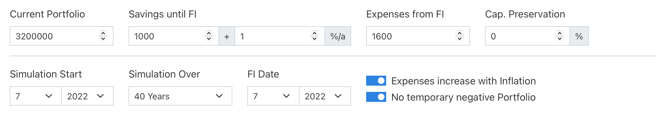
Clara is a successful entrepreneur and has now sold her company at the age of 60 to take her well-deserved retirement. As she has been self-employed all her working life, she has not paid any contributions into the public pension fund and would therefore like to cover her living expenses entirely from withdrawals from a broadly diversified equity portfolio. Through the sale of her company, this portfolio has now grown to a value of 3.2M$.

In order to also cover the longevity risk, Clara therefore runs a simulation over 40 years, i.e. until her calculated 100th birthday:

We now look directly at the calculated withdrawal rates on the 2nd tab:

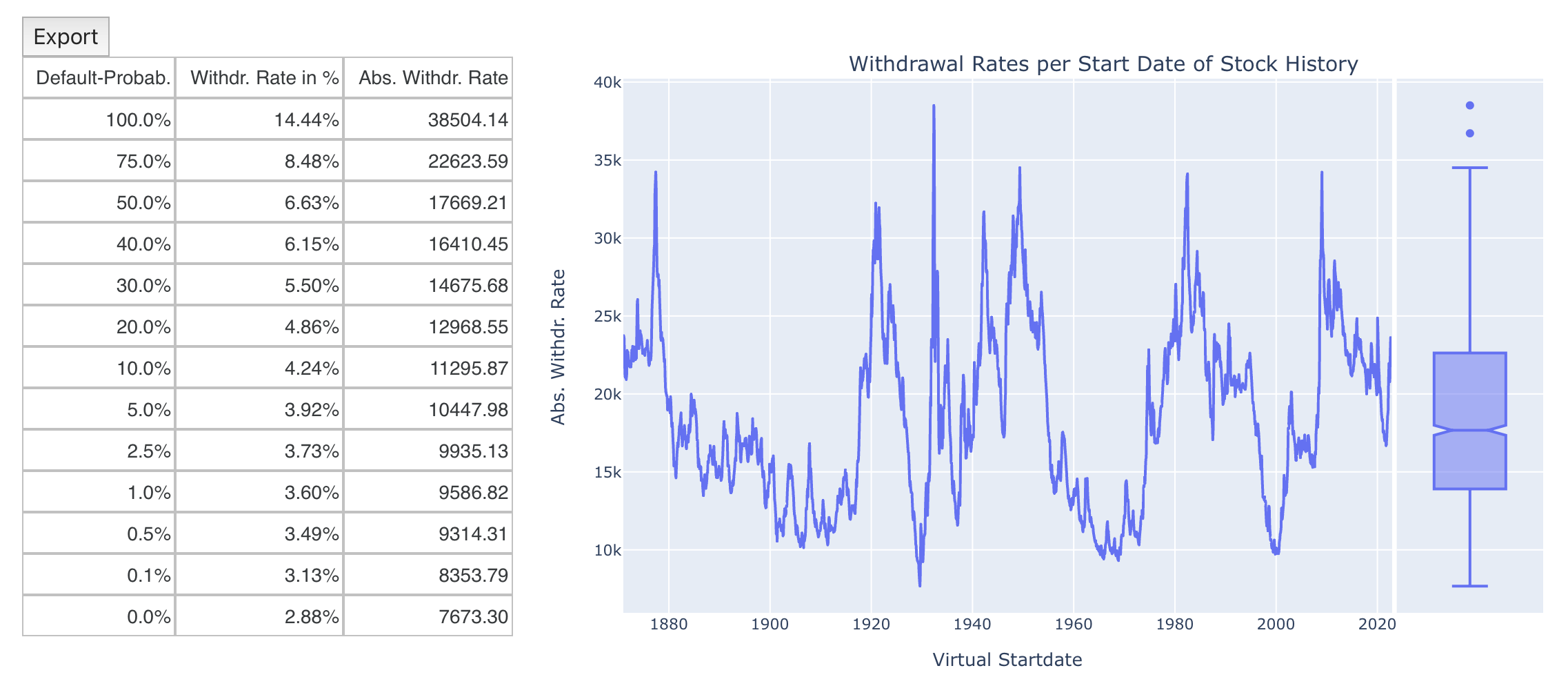
Clara would be able to withdraw inflation-adusted $7,673 per month until her 100th birthday without going broke even once in the last 150 years. A nice result, which should allow her therefore a comfortable retirement.

Nevertheless, a worst-case scenario would result in her portfolio being completely depleted at the end of the 40-year simulation period. However, Clara would like to manage her assets in such a way that her two children are also provided for after her death. She therefore wonders if there is a way to calculate monthly withdrawal rates in such a way that the portfolio is not completely depleted at the end but instead keeps a certain target amount at the end. The simulator offers the field “capital preservation”, which allows exactly this. Clara sets the capital preservation to 100%, i.e. at the end of the observation period the portfolio should remain at the initial level even in the worst case. If we look at the calculated withdrawal rates, we see that the difference is not that dramatic:

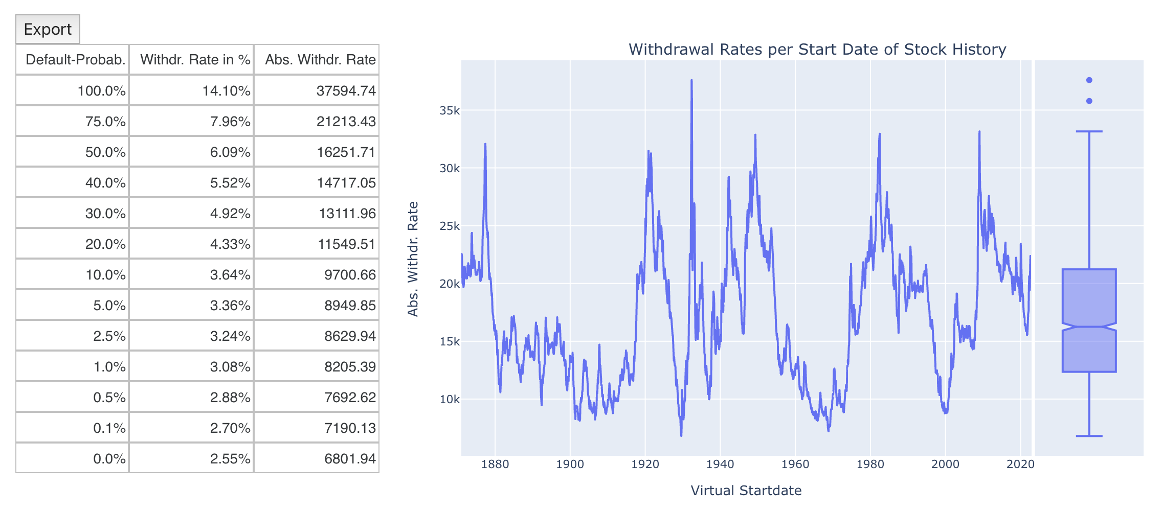
Instead of $7,673, Clara would still be able to withdraw $6,802 per month and maintain her capital in full. Let’s now enter the $6,802 in the “Expenses from FI” field and look at the prediction of the portfolio development. In the worst case, the depot balance is no longer zero but in this case nominally 6.8M$. The keyword “nominal” already indicates that here the inflation-related increase must be considered. If we hide this with the switch “Real values without inflation increase”, we see the following picture:

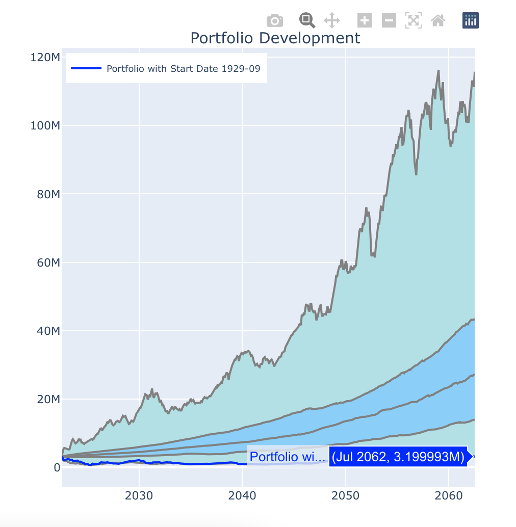
This means that the final balance of the portfolio at the end of the simulation period is again exactly real 3.2M$ in the worst case. As desired by Clara, her assets are therefore preserved in real terms and she has done everything to secure her assets for the next generation.

If you want to follow the example directly, you can find the corresponding json file here. If you want to be notified about new posts, please use your favorite RSS reader and subscribe to this blog using the RSS link in the main navigation bar or through this link.