Virtual Case Study: Ben

Today, in another virtual case study, I want to show pitfalls that can happen when calculating withdrawal rates with high future incomes. As usual, I recommend running the case in parallel on the simulator. For those who want to load the full example directly into the simulator, the link is at the end of this article.

Ben turned 55 this year and has been considering retirement for some time. He has already saved up a nice stock portfolio during his working life, currently worth 500,000€, and is also entitled to a pension. More importantly, however, he has a large life insurance policy that will bring him a payout of a round million $ on his 65th birthday in January 2032. Ben now wants to calculate precisely what level of spending this constellation will allow him if he retires now. Ben chooses 45 years as the simulation period to also cover the longevity risk, i.e. the simulator then calculates monthly expenses that would theoretically last until his 100th birthday.

Ben therefore makes the following entries in the simulator:

At first glance, the forecast of the portfolio development already looks encouraging:

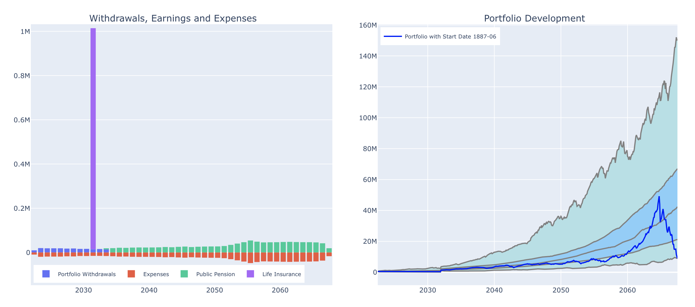
The income and expenses overview is of course dominated by the life insurance payout in 10 years. The $1,600 expenses per month entered by default would already be fully covered by his public pension from 2034 onward and it can be seen that his portfolio would grow strongly in all historical trajectories. So there is obviously a lot of potential here to increase the monthly spending level significantly. For this purpose, we now look at the calculated withdrawal rates in the 2nd tab:

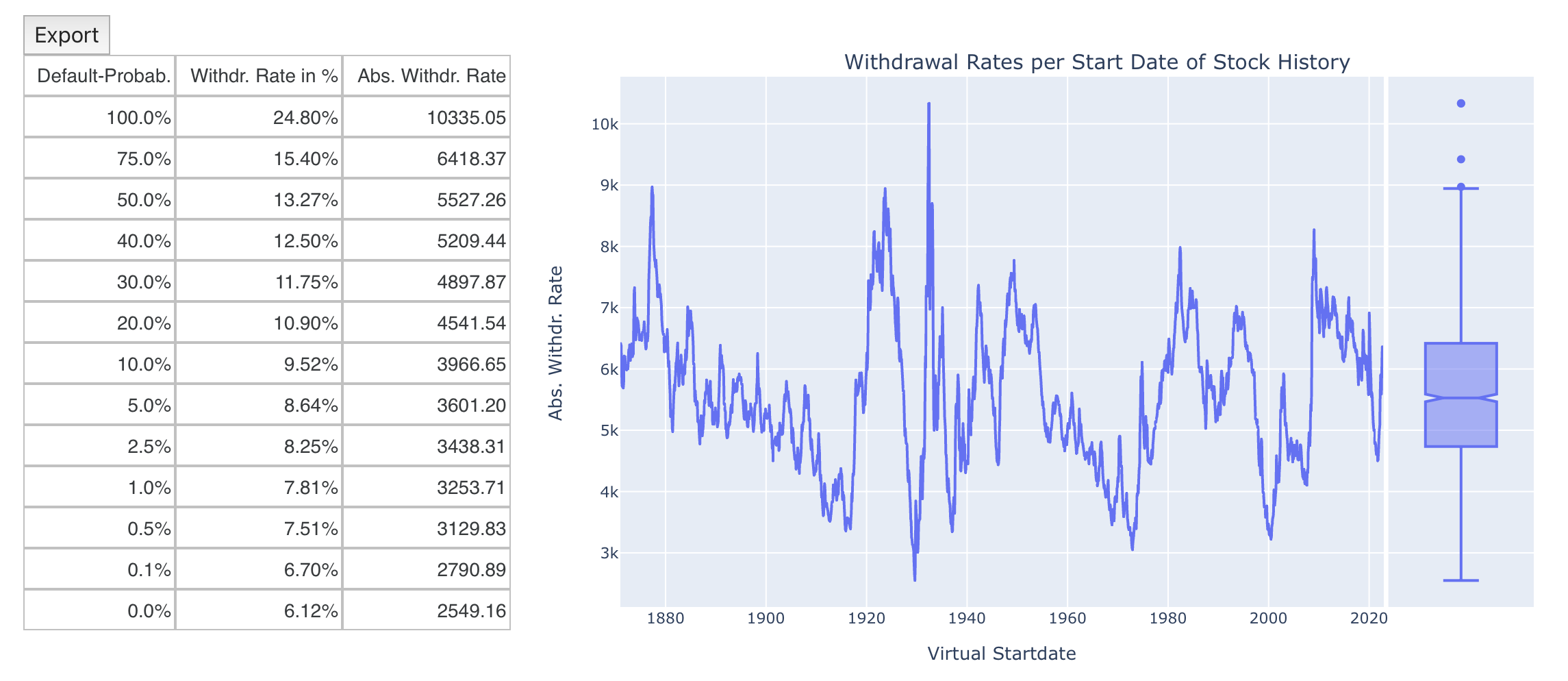
Accordingly, Ben could withdraw inflation-protected $2549.16 per month from his portfolio starting immediately and, according to all historical market trends, would not run the risk of going broke prematurely. Nevertheless, Ben is somewhat disappointed. He had actually expected that the large payout on his life insurance policy in 2032 would allow him to take out a much higher withdrawal rate. What happened here? Let’s enter the $2549.16 as “Expenses from FI” and take a closer look at the forecast of the portfolio development:

Even in the worst case shown, Ben would still have 7.3M€ in the portfolio at the end of the simulation period. However, the calculated withdrawal rate in the worst case should actually ensure that the portfolio is completely depleted, i.e. that it ends up exactly at zero at the end of the simulation period. Is Ben still giving away potential here?

The solution lies in the switch “No temporary negative portfolio”, which is always set by default. If we go back to the calculation of the withdrawal rates and remove this switch, the calculated values will immediately change significantly:

So suddenly even the withdrawal of $4252.37 per month would be possible without any risk of bankruptcy? Of course, that would be much more to Ben’s taste. However, there is a catch. We can see it if we now enter these $4252.37 as “Expenses from FI” again and look at the portfolio development: Now the worst case in 2067 actually ends at zero as expected, but the pitfall lies in the portfolio development shortly before the payout of the life insurance in 2032. A zoom into this area looks as follows:

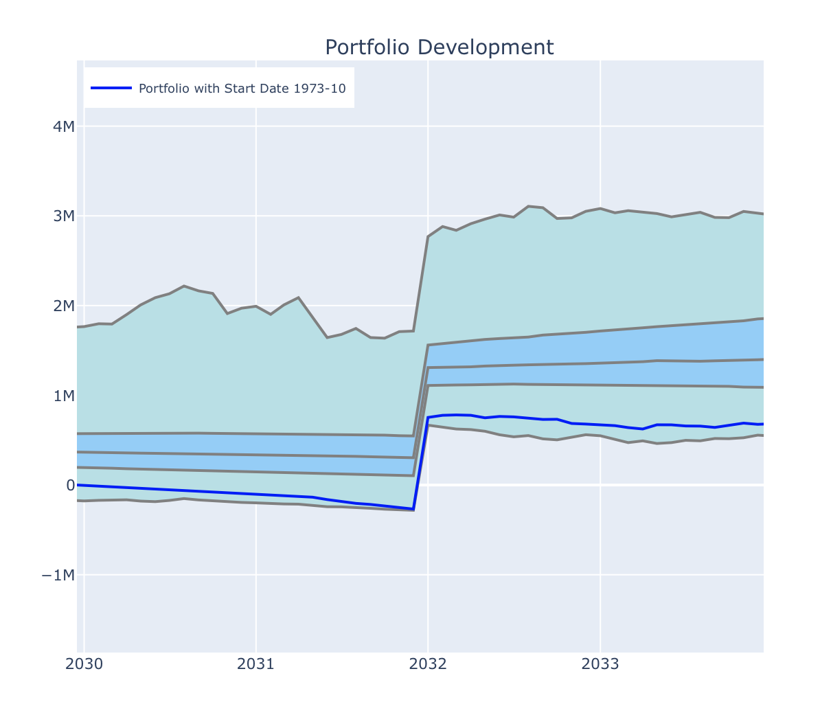
You can see nicely the payout of the life insurance in January 2032, which leads to a jump upwards in all historical portfolio developments. In the worst case, however, the portfolio becomes negative until the payout arrives, i.e. in this phase Ben would not only have to sell his portfolio completely, but he would even have to borrow money from the bank at the interest rate that corresponds to the current return rate of the stock market. This sounds a bit crude, of course, and is simply because of the way how these withdrawal rates are calculated mathematically.

Ben therefore faces a dilemma: If he chooses the higher withdrawal rate, he would have to borrow money at a certain point in time, but he would then be able to deplete his portfolio completely and would have also optimized his standard of living. If he chooses the lower withdrawal rate, he can be sure that his portfolio will never become negative. However, then he will not be able to use his entire portfolio and will feel that he is living more frugally in retirement than is actually necessary.

Unfortunately, there is no simple solution to this problem and Ben has to find a compromise between these two possibilities. For all readers, it should at least remain in the back of your mind that the switch “No temporary negative Portfolio” exists at all. In most cases, it will show no difference in the calculated withdrawal rates. However, if large cashflows are expected in the future, it is worthwhile to check if there are any differences. It is also important to note that all publicly available FI calculators that I know of do not have this option and always show the higher withdrawal rate. If one does not know the effect shown here, trusting their numbers therefore might be a little dangerous.

If you want to directly load the example analysis you can find the necessary json-file here. If you want to be notified about new posts, please use your favorite RSS reader and subscribe to this blog using the RSS link in the main navigation bar or through this link.