Integration of historical German stock and inflation data.
After a long summer break I am back today with a hopefully interesting topic. A few months ago I discovered the following book from 1993: “Können Aktienkurse noch steigen? - Langfristige Trendanalyse des deutschen Aktienmarktes” by Gregor Gielen. In this book the author describes a historical index of the German stock market since 1870(!) even with dividend and inflation data, i.e. Gielen develops a complete performance index. I have updated this index with current data of the CDAX as well as inflation data of the German Federal Statistical Office until today and integrated it into the simulator as an alternative data basis.
One motivation for this was that the focus on the American S&P 500 data for the calculation of safe withdrawal rates has bothered me for some time. For one thing, the inflation data come from the U.S. consumer price index, i.e., they are not directly comparable to other countries. For another, the historical performance of the U.S. stock market is also slightly better than all other developed countries. Therefore, for a more realistic analysis of withdrawal rates in the non-U.S. region, other data are actually needed, but are not easy to obtain. There are some commercial providers of such data, but their prices are steep, and they usually carry a very restrictive license. An integration of such data into my free simulator is therefore difficult.
Nevertheless, I see the integration of long-term data of the German stock market now as a first step towards a better quantitative understanding of withdrawal rates outside the US economic area. Let us first look at the data itself and how I have tried to prepare it for the simulator.
German Hyperinflation in 1923, currency reform in 1948 and link to the current CDAX
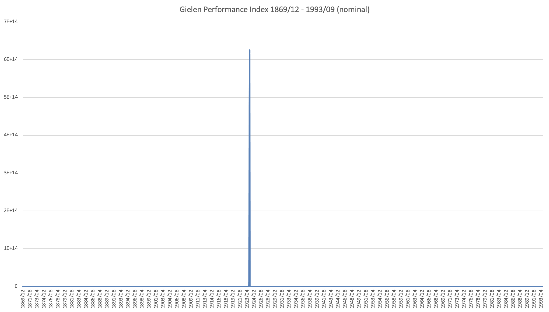
When I first looked at Gielen’s nominal price data in Excel, I had to laugh at first. As you can see, you see nothing:
If you display the Y-axis logarithmically, then the picture becomes somewhat clearer:
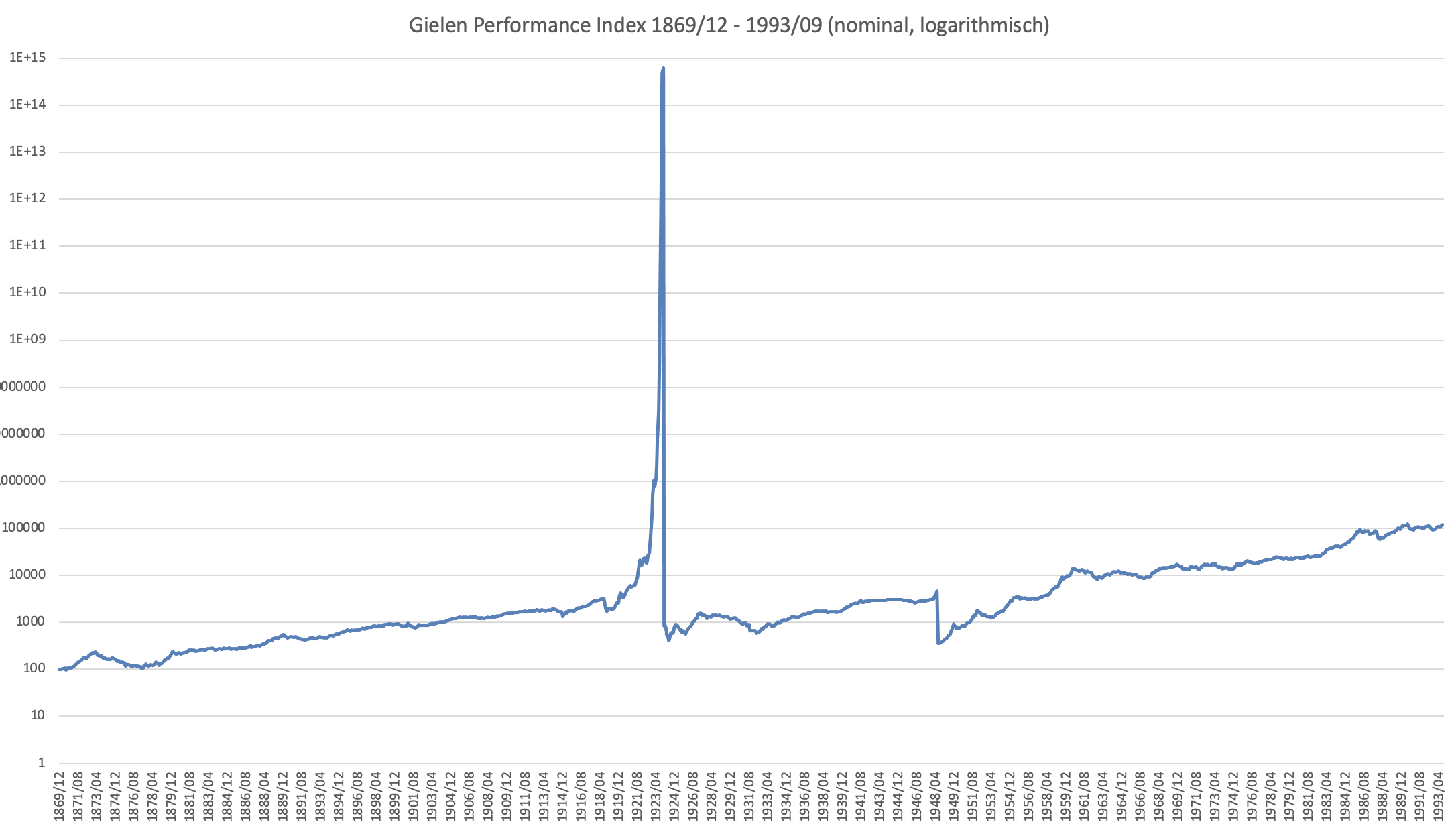
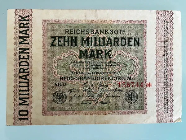
The “tiny bump” in the data is the peak of the German hyperinflation in December 1923. There, according to Gielen, the stock index reaches a value of 6.3*10^14(!) in the then valid currency Papiermark. The cover picture of this article appropriately shows an original cash-bill valued at 10 billion Papiermark from October 1923. At that time, all Germans were mathematically a nation of billionaires, but unfortunately it was a time of poverty and extreme discontent, which ultimately then contributed to the next catastrophe from 1933.
The absolute values of the index from this period are certainly not exact and can only approximate the situation at that time. My first reaction was therefore to use these data only after the currency conversion to Reichsmark or Rentenmark in January 1924. After thinking about it for a while, however, I decided against it. On the one hand, one would no longer see all the effects of the First World War, on the other hand, such a hyperinflation is a rare but nevertheless a realistic extreme event and it would be interesting to examine how such an event would affect our thoughts on financial independence (and also we are again in a time of relatively high inflation). I therefore tried another way and converted all index and inflation values before December 1923 into the new currency Rentenmark. Since one Rentenmark was equal to one trillion Papiermarks, this means dividing all older index values by the factor 10^12, i.e. a 1 with 12 zeros!
The currency reform in 1948 in West Germany leads to further uncertainties in the data due to stock exchange closures and completely unclear ownership of the shares. Gielen nevertheless dares to construct a continuous index over this period and describes his approach in detail in his book. As a result, you can see in the index a drastic slump of over 90%(!) in mid-1948, which roughly matches the approximate exchange ratio of 10 Reichsmarks to one D-Mark that was applied to cash. This collaps of the index-value drastically shows the impact that World War II had on the German economy.
Gielen continued his index until September 1993, which was the editorial deadline for his book. For the continuation of this index, which was constructed as broadly as possible, into the present day, I did not use the DAX, but the CDAX Performance Index. Instead of the 30 largest stocks, this index contains all General Standard and Prime Standard stocks traded in Frankfurt, currently more than 400 stocks. The CDAX was introduced exactly like the Dax at the end of 1987 and there are even data series of the Bundesbank, which calculate this index back to the beginning of 1970. This raises the question of how best to combine Gielen’s data with the new CDAX data. An analysis of the back-calculated values 1970-1987 showed that their performance deviated strongly from Gielen’s index. I therefore suspect that this back-calculation only used the stock prices of the individual stocks included in 1987 but did not make a true simulation of the index with corresponding company shifts. However, I am not sure about this. Between 1987 and 1993, i.e. during the common period of Gielen’s index and the CDAX, the performance data agree relatively well, so that in the end I decided to use Gielen’s data until September 1993 and the CDAX from October 1993 on and to link it seamlessly to the end of Gielen’s index. For the inflation data from 1993 onwards, I have analogously taken the official data of the German Federal Statistical Office, so that in the end I get continuous and hopefully consistent data series for a performance index of the German stock market and for inflation from January 1870 to September 2022 in the current currency euro. By the way, if you want to have a look at Gielen’s index in detail, you can find most of the data after registering at https://histat.gesis.org. There you will also find other very interesting historical German data series including the respective source references.
Long-term real performance of this index
Looking at the graphs of the nominal performance index and inflation, the extreme effect of hyperinflation is of course noticeable at first, even in the logarithmic representation. Nevertheless, the peaks in the index and inflation could already be a first indication that a (hypothetical) investor in this stock index may have been somewhat protected from the extreme effects of inflation, at least compared to investors in bonds, who were wiped out after the currency changeover in 1923. To examine this in more detail, let’s completely ignore inflation in the following chart and instead look at the real performance index, which tracks the inflation-adjusted returns. This index now looks comparatively harmless and is worth a more detailed look:
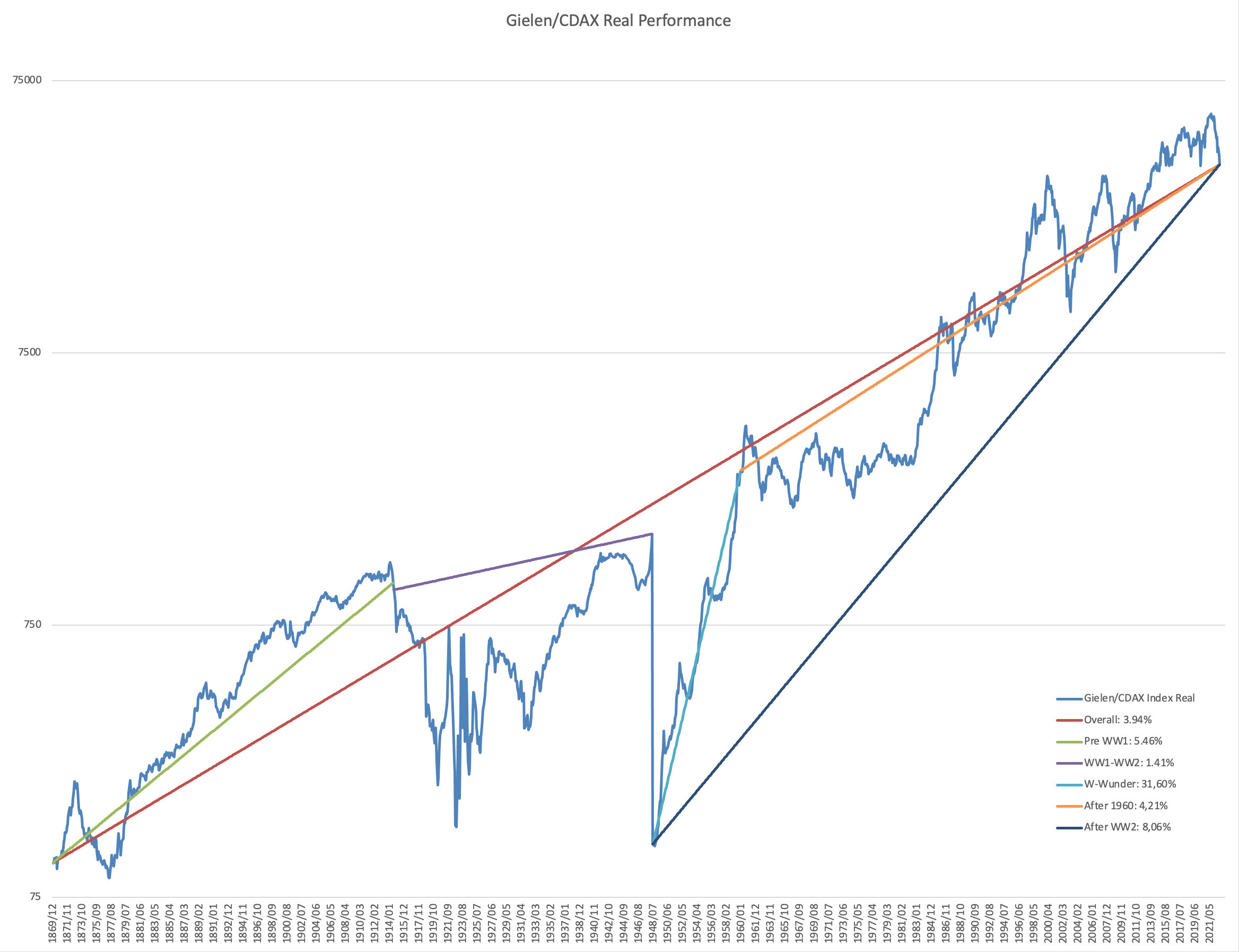
You can see lines of constant average return, which I have added somewhat arbitrarily for certain phases of the index. I have drawn the first line from the beginning of the index at the end of December 1869 until the outbreak of World War I in July 1914, where the index achieved an average performance of 5.46% annually after inflation. Between July 1914 and the second currency reform in July 1948, I have drawn another performance line, showing above all the effect of the two world wars and the hyperinflation. Not surprisingly, the average performance of 1.41% is significantly smaller there and it would even have been negative if I had included the over 90% collapse due to the 2nd currency reform there. After the currency reform until about the beginning of 1960, I have drawn in another phase, which describes the so called German “Wirtschaftswunder” or “economic miracle”. During this period, an investor would have achieved a whopping 31.60% annual return after inflation. After that, logically, the curve flattened out again and between the beginning of 1960 and today achieved an average performance of only 4.21%, significantly less than the average performance of the U.S. stock market with about 6.6% annual return after inflation. As mentioned above, however, the definition of such periods is highly subjective. If one takes the performance from the beginning of 1960 until today, i.e. including the German economic miracle, then this would give an annual return of 8.06%, for example.
What surprised me most about this data, however, was the overall performance of the index from 1870 to the present. Despite losing two world wars and having two failed currencies, a (hypothetical) investor in this index would still have earned an annual average return of 3.94% after subtracting inflation over the entire period!
First results in the simulator
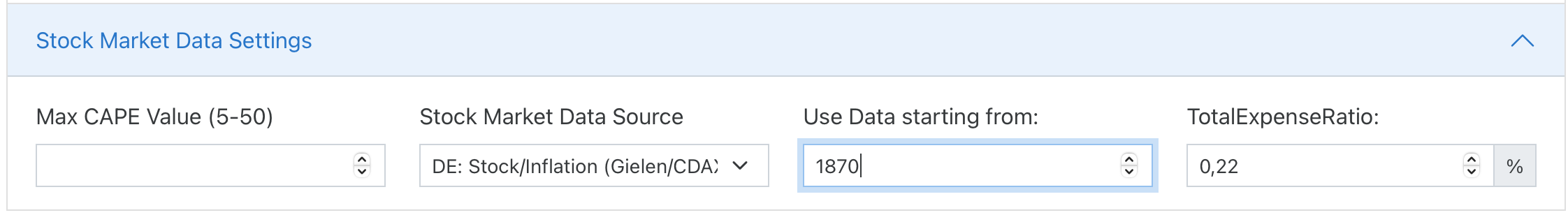
I have added this data to the simulator for a few days. They can be accessed via the “Stock Market Data Settings” tab. In addition to the default value of the US S&P 500 and inflation data from Rober Shiller, the data series described above with the performance index from Gregor Gielen and the CDAX together with German inflation data can now be used there as an alternative selection.
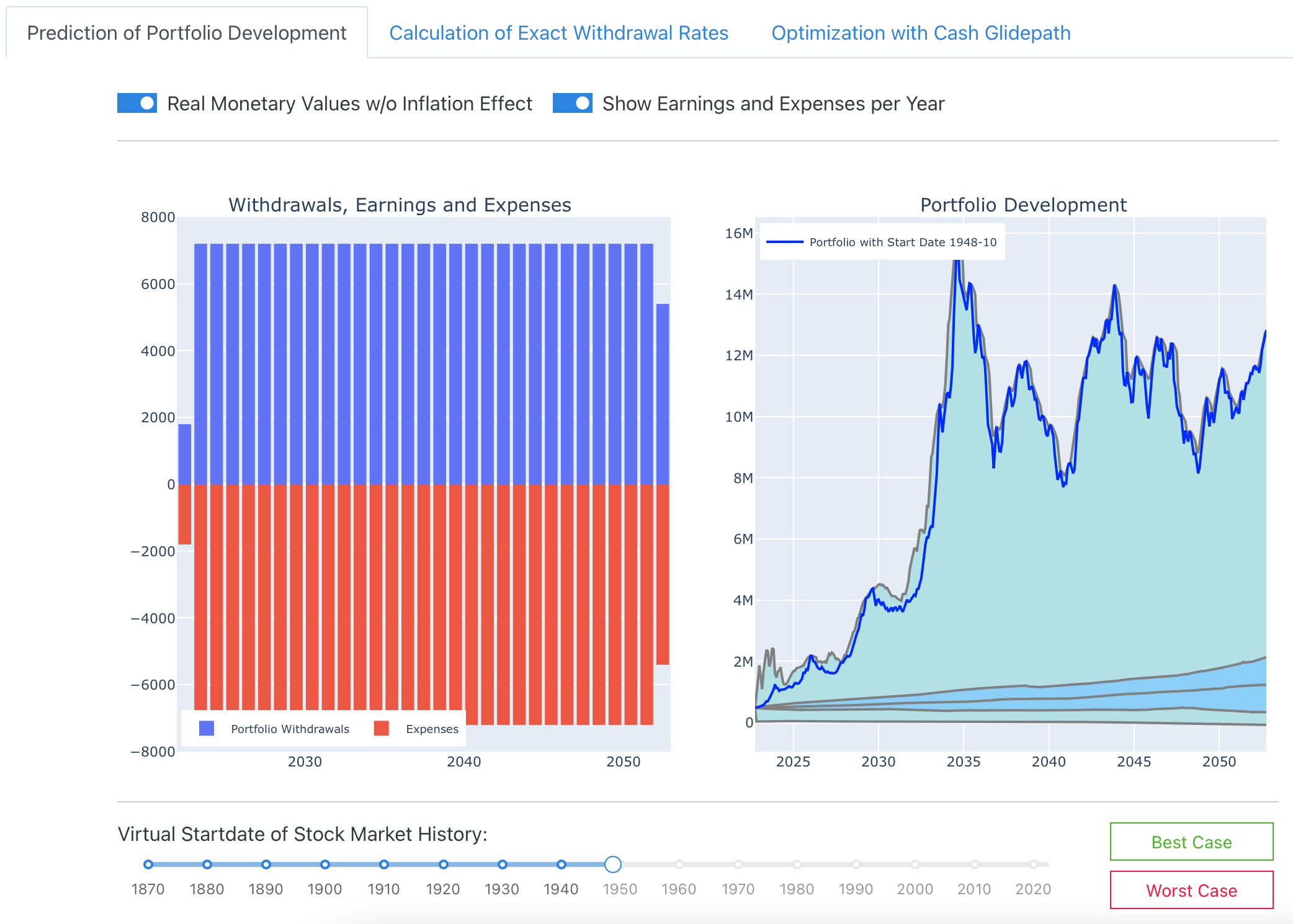
To begin, let’s look at how our standard trinity example looks with this price data. To use all available data points, I set “Use data starting from” to 1870, since we now have even one year older data for Germany:
The historical simulation of the portfolio development over time now looks rather scary: Our monthly withdrawals of $1,600 from our stock portfolio of $480,000 according to the 4% rule apparently lead to disaster very quickly with the default settings:
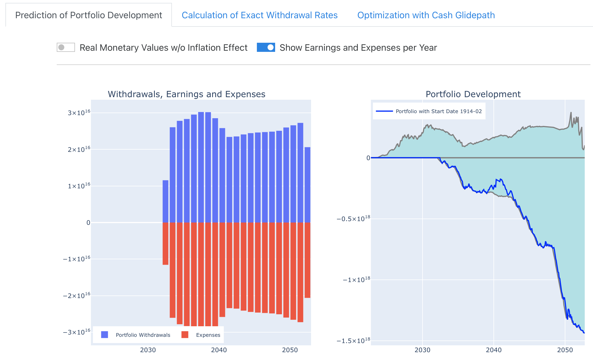
If you look at the left graph of withdrawals, Earnings and Expenses, you can quickly see the cause of the problem: We start the simulation in October 2022. In the historical worst case (according to the right graph corresponding to a virtual start date of our stock history in February 1914), the annual expenses from July 2032 (corresponding to the virtual date of December 1923) would suddenly increase to gigantic orders of magnitude, which make all income and expenses before that appear so tiny that they are not even recognizable on the graph. Obviously, we are just seeing the effect of the hyperinflation of 1923 here. We remember that by default, the switch “Expenses increase with Inflation” is set in the simulator. This switch now ensures that we want to maintain our monthly expenses of $1,600 even through a hyperinflation, which then leads to the simulator withdrawing extreme amounts from our deposit every month from then on. Despite the above described real 3.94% return of the German stock market in the long-term average, a 4% rule is of course not sustainable here.
Nevertheless, let’s have a look at the exactly calculated withdrawal rates on the 2nd tab:
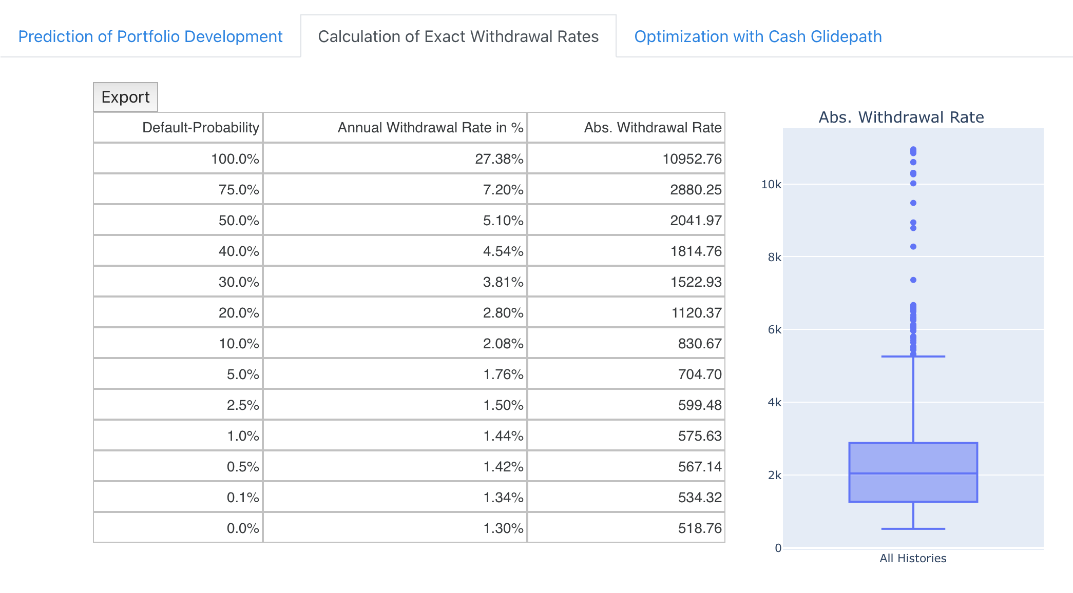
The long-term safe withdrawal rate of the German stock market for a 30-year withdrawal period is apparently only 1.3%. If we accept a probability of bankruptcy of approx. 2.5% analogous to the traditional 4% rule of the U.S. market, we would thus only be allowed to declare a 1.5% rule for the German stock market. If we enter the corresponding monthly expenses of approx. $600 back into the first tab as “Expenses from FI” we see the following picture:
Although there is a remaining probability of bankruptcy and the worst case therefore remains negative after 30 years, the majority of historical developments now actually lead to a positive end result. This is remarkable because, in purely mathematical terms, we would be able to completely compensate for even a renewed hyperinflation analogous to 1923 by increasing the monthly withdrawals accordingly without going bankrupt (at least in the vast majority of cases). However, at this point I would like to point out the following: The calculations that the simulator has to perform here are numerically much “shakier” than the normal cases that we have calculated so far. After all, the numerical values before and after hyperinflation are 12 orders of magnitude apart. It would therefore not surprise me if there are at least significant rounding errors here. In the worst case, there are even unrecognized calculation errors here, which only manifest themselves in such extreme situations.
Furthermore, we are talking about a very artificial model here: In real life, such a withdrawal plan would be prone to failure because the stock exchanges would have been temporarily closed and regular trading was often not possible at all. Not to mention all the other human tragedies and catastrophes of that time, which are hidden behind these bare numbers.
On the other hand, the results of the simulator here seem basically plausible to me. However, I would be very happy to receive comments, suggestions how you see this.
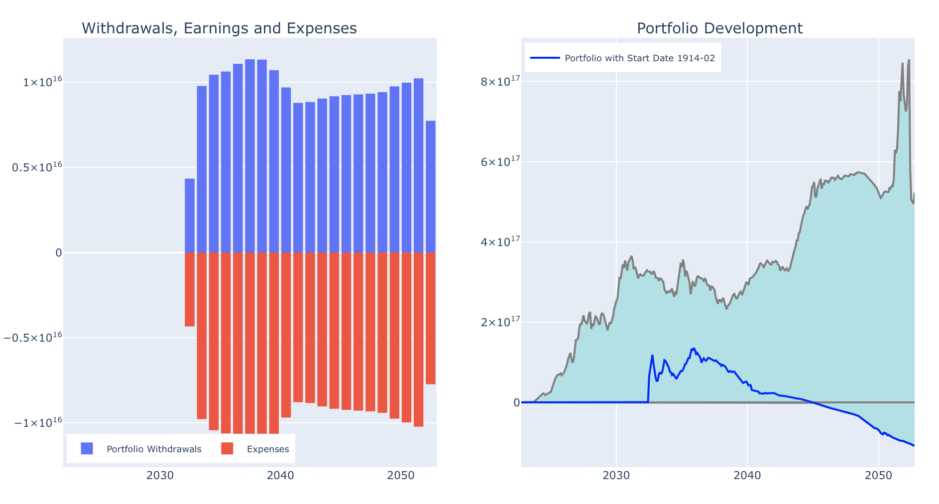
As a last step in this article, we now set the switch “Real Monetary Values w/o Inflation Effect” to be able to focus on the real returns. All effects of inflation and hyperinflation in 1923 are now hidden. Therefore, the simulator result actually looks relatively “normal” again now. If we look at the “best case” instead of the usual worst case by pressing the respective button, we now see the following picture:
As might be expected, the best-case would start shortly after the completion of the second currency reform in October 1948 and would go along with the complete “Wirtschaftswunder”.
Outlook and request for support
Hopefully, this article will be the starting point of a somewhat longer series. As indicated above, I have a medium-term goal of calculating safe withdrawal rates much more generally, i.e., without the focus on U.S. equities and U.S. inflation. One of the next steps towards this will also be to allow a separate selection of stock and inflation data in the simulator. For example, it would be interesting as a German user of the simulator to always use the German inflation data, since all expenses are ultimately influenced by them. Completely independent of this, however, this German investor can then decide whether he or she would prefer to use a stock portfolio with US or German stocks. From the comparison of corresponding withdrawal rates, some interesting information should be derived, not least an estimation of safe withdrawal rates of a real globally diversified portfolio.
At this point I would also like to start a small request for support: The speed with which I am progressing here is limited by the access to corresponding price and inflation data. So if any reader of this blog knows a good source for historical inflation and index data, e.g. for other European countries, I would be very happy to receive a hint. Ideally, the data should also be available as monthly data to enable precise calculations and, of course, there should be no licensing problems in using the data. An integration of such data series is then relatively straightforward and would then also allow users from these countries an analysis with reference to their home stock market or at least their home inflation data. Thanks a lot in advance!
This brings me to the end of today’s article and I hope that the content was interesting. If you want to do your own analysis on withdrawal rates of the German stock market, you can do it now in the simulator. If you want to ignore the hyperinflation, you can simply restrict the price history to the years from 1924 onwards, then the results will not look quite so scary. Feel free to share interesting findings as comments below, I would be happy.
If you want to be notified about new posts, please use your favorite RSS reader and subscribe to this blog using the RSS link in the main navigation bar or through this link.