Safe Withdrawal Rates are heavily influenced by Other Cashflows.

Everyones personal finance situation is different. When calculating withdrawal rates from a stock portfolio, this holds especially true. If, for example, in addition to having the stock portfolio you are entitled to receive public or corporate pensions, a straightforward application of the 4% rule typically leads to the following situation: In our “Trinity standard example”, we could withdraw a (relatively) safe $1,600 per month from our portfolio of $480,000. Although these $1,600 are already inflation-adjusted, it would of course not allow for a luxurious lifestyle (especially since this amount is also before taxes!). Nevertheless our “example-retiree” at age 60 decides to retire now anyway, because he expects some public and corporate pensions later. In particular he is entitled to a generous company pension of $1,400 starting from 65 and a public pension of, say, $1,801 after his 67th birthday (don’t worry about the odd amount, this corresponds to exactly 50 germany pension points so I keep this value to be consistent with the german example). From this point on his income suddenly amounts to approx. $4,801 monthly and after the past 5-7 “frugal” years our retiree suddenly doesn’t know what to do with all that money. Couldn’t he have planned a better withdrawal-strategy to keep his standard of living more constant over the years?

The simulator can take a large number of additional “cash flows” into account

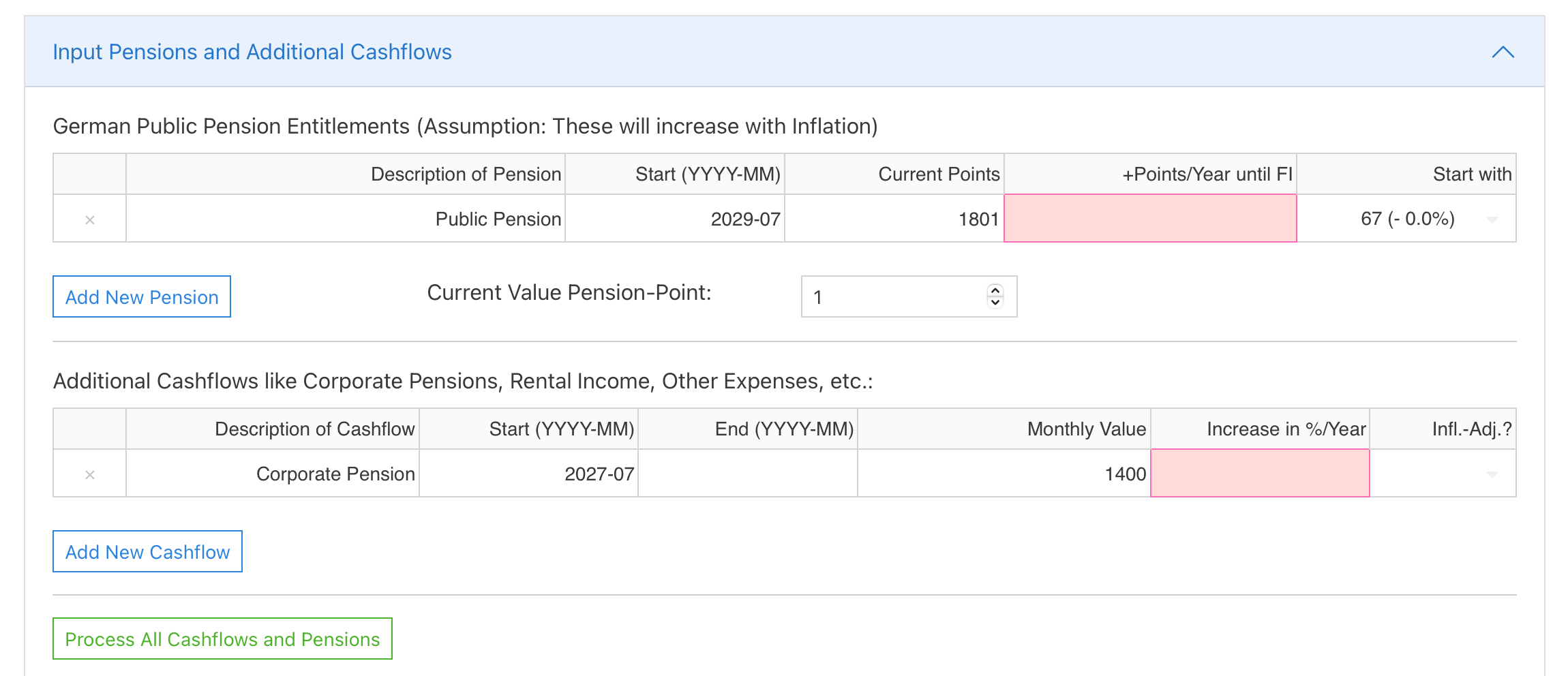
Now let’s look at how this can be done in the simulator. As usual, I recommend to start the simulator in parallel in a 2nd browser tab while reading, to be able to “play through” the example in parallel. To do this, please download the following example analysis and then click the button “Load Analysis” and chose the file you have just downloaded. All input parameters should be filled correctly now and if you open the tab “Input Pensions and Additional Cashflows” you should see the following additional entries:

Now a word of caution: Especially this section is heavily influenced by the German public pension system which is point-based. I will try to work around that for our more international readers and hope that the end-result will not be too confusing. To this end the default values of the english version of this example are slightly different and start with a pension-point value of 1.

The first section allow us to enter public pension entitlements. We have entered a value of 1801 here in the field “Current Points” to be exactly consistent with the german example figures. This corresponds to a monthly pension of $1801 with a pension point value of 1. Since retirement starts immediately, no more additional points will be earned annually until then, so we leave the field “+Points/year until FI” empty. Our example retiree just turned 60 in June 2022, so will receive the full public pension without deductions at 67 therefore starting in July 2029 (again this is based on the German system. If your system is different, choose the date accordingly). We therefore enter 2029-07 as the start in exactly this format. (Another warning: The simulator does not do a thorough validation of the input, i.e. if you want to enter random gibberish there you can do so and the simulator will not really complain. However, the calculation later will most probably not work. If in doubt compare your input with the screenshot above). It is important to set the last field to “67 (-0.0%)”, because the public pension in this example should start without deductions. If you would use one of the other entries, these would correspond to claiming the public pension earlier, e.g. already at the age of 63, but at the price of monthly deductions in this case of 14.4%. After that, the value of a pension point of $1 is already set by default for our international audience. Only change this if you know what you are doing.

In contrast to all other input fields, the entries in this “Cashflows” tab will not be processed until the “Process cashflows and pensions” button is pressed at the bottom. Otherwise, every single field change would trigger a pointless re-calculation on the server and would consume unnecessarily capacity. Before we press this button, however, we want to complete the example and enter the company pension there as well: The table below the pension rows is used for this purpose and already contains the necessary line. We designate this cash flow in the first field as “Corporate Pension” and set 2027-07 as the start month, since this pays out from the assumed age of 65. The field “End (YYYY-MM)” remains empty, so the simulator always will include this contribution until the end of the simulation period (Hint: If cashflows are to start immediately but only run until a certain point in time, the field “Start (YYYY-MM)” can remain empty and only the endmonth must be set accordingly). Monthly amount should be, according to the example, $1.400. Normally in Germany, company pensions must be increased annually, e.g. by 1%, which we could then enter in the next field. In our simplified example, however, we leave the field empty. Last but not least: In the last field we can specify that the cashflow will be adjusted with inflation. For company pensions this is usually not the case so in our example we also leave this field empty.

Normally we need have to press the button “Process All Cashflows and Pensions” now to make sure that all of these entries are processed correctly. Since we have “cheated” and simply loaded the example file, this has happened already (but pressing the button again doesn’t hurt). Now the following overview of Withdrawls, Earnings and Expenses as well as the Portfolio Development appears, as usual with the “worst case” of all possible historical developments shown in dark blue on the right hand side:

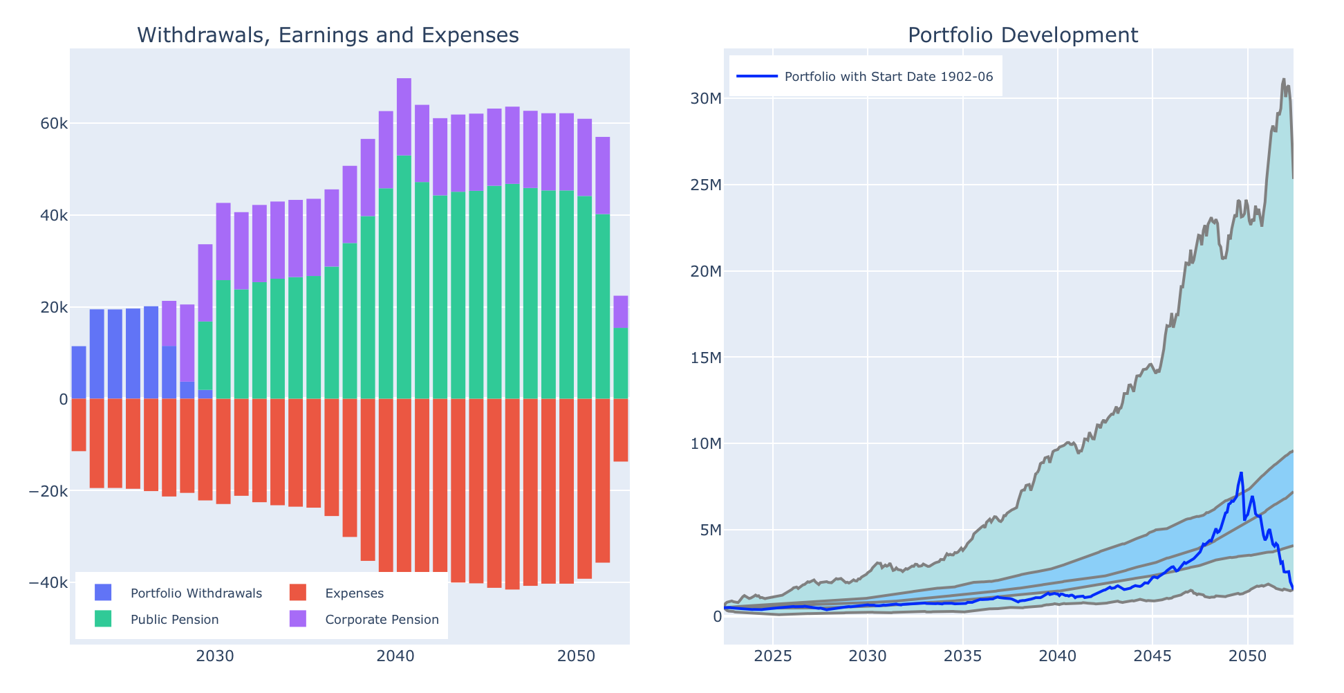
The overview of withdrawals, earnings and expenses has changed completely now: All additional cashflows now appear above the horizontal line representating the different income-streams, each separated by color. You can see in particular that the portfolio withdrawals (in blue) already stop in the year 2029, after which the public pension as well as the corporate pension are completely sufficient to cover the monthly expenses of $1,600. Not only that, but you can also see that after 2029 all income streams will significantly exceed the expenses (as usual shown below the horizontal line in red). Thus, from this point on, nothing will be withdrawn from the portfolio and instead the excess money will be invested into our portfolio every month (Reminder: The simulator currently operates internally with a 100% stock quota, i.e. assumes that we are fully invested in the stock market at all times. The only exception are the so-called cash glidepath calculations in the 3rd tab, which will be explained later). This also means that the portfolio grows with the stock market from this point on and we can see this in the portfolio development even in the worst case shown. If we look at the final value of the worst case we see that the portfolio end at over 1.5M$.

However, this implies that our “example retiree” keeps his frugal lifestyle of the first 5-7 years of retirement even after the start of the public and company pensions. But of course this was exactly not what we intended to do by this exercise. Instead, we wanted to use the simulator to calculate optimal withdrawal rates that take the additional later cash flows into account and allow for an earlier withdrawal of higher monthly amounts. We could now enter such higher withdrawal amounts in the field “Monthly expenses starting from FI year” on a test basis and figure out the optimum by iteration. However, it is much easier if we look at the exactly calculated withdrawal rates directly on the 2nd tab. All cash flow entries are automatically taken into account there and we should now see the following picture if we go to the second tab:

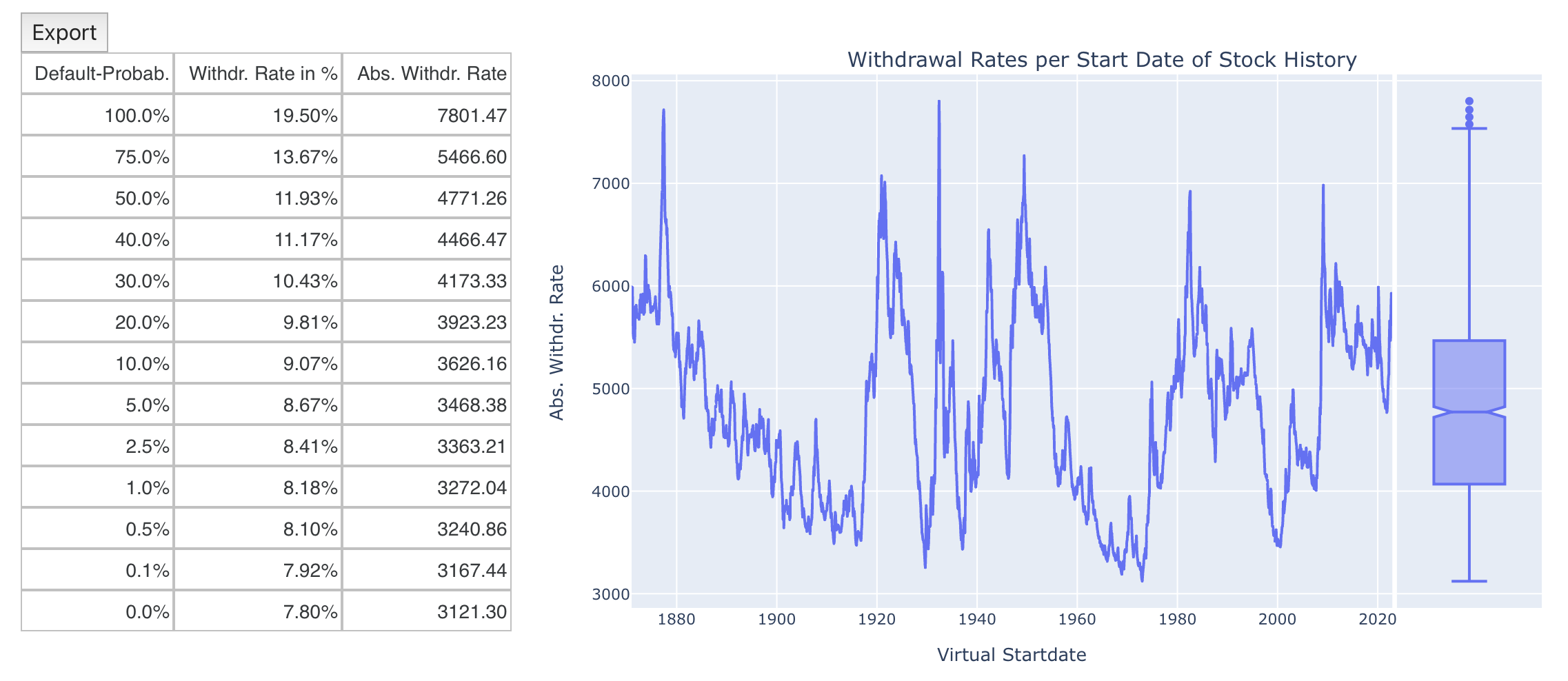
The safe withdrawal rate with 0% probability of bankruptcy is now $3,121 per month compared to the original $1,600 per month. If we want to allow ourselves a small residual risk of 2.5% (analogous to the original 4% rule), we could even withdraw $3,362 per month until the end of the simulation period of 30 years and would thus have achieved our goal of better planning of withdrawals, especially because these withdrawals are also inflation-adjusted in the default setting, i.e. they grow with inflation, as can also be seen in the expenses overview. The middle column in the table converts the absolute withdrawal rates into annual percentage withdrawal rates with reference to the starting value of the portfolio. There you can also see that the additional cashflows now lead to much higher relative withdrawal rates.

At this point, another important remark: The simulator assumes that the German public pensions grow with inflation (which can be seen in the development of the green bars in the overview). Of course, this is only an assumption and one could make more optimistic or more pessimistic assumptions which are equally valid. If necessary, I might add a “correction factor” later, which will then allow to adjust the relation with inflation a bit. Keeping this in mind, another interesting effect can be seen in the overview of income and expenses (in the 1st tab): Due to the inflation adjustment, the relative share of the public pension in the income compared to the company pension (which remains nominally constant in our example) becomes significantly higher over time. This effect becomes even more visible the longer the simulation period is.

Finally, we now enter the above-mentioned safe withdrawal rate of 3,121€ per month back into the “Expenses from FI” field and look at the overall situation again:

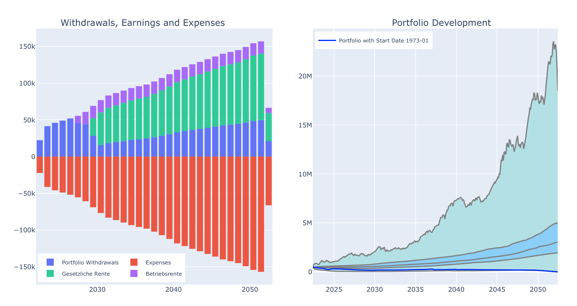
In the worst case scenario we now end up at 0 at the end of the simulation period, exactly as desired. And the box plot over all histories correspondingly also has its minimum there. We can see in the overview of withdrawals, earnings and expenses that we have actually reached an optimum with this withdrawal rate: The portfolio withdrawals (in blue) are fully needed in the beginning to cover the monthly expenses, then the company pension and the statutory pension start successively, so that the portfolio withdrawals may become smaller accordingly. All in all, we now use our stock portfolio better and more evenly until the end of the simulation period, which is exactly what we wanted to achieve.