Why is the consideration of inflation so important?
When considering financial freedom, there is one issue that cannot be ignored, and that is inflation. After all, our financial planning typically extends decades into the future. Anyone in their 50s who is seriously considering FIRE still has an average life expectancy of around 40 years ahead of them and should therefore definitely take into account that, assuming an average inflation rate of 2.5% per year, each Dollar will only be worth about 36 cents in 40 years. As can be seen at the moment, there will also be phases in the meantime in which inflation is significantly higher. This was also the case in the 1970s, for example. On the other hand, there were also phases with significant deflation, e.g. after the peak of the Great Depression in 1929. Anyone who ignores such effects therefore runs the risk that purchasing power will drop noticeably in old age and financial freedom will suffer as a result.
Nominal or real values?
The simulator calculates internally with so-called nominal values, i.e. the development of the portfolio uses the price data of the broad american S&P 500 index. In the default setting, all portfolio values shown in the first tab thus always include inflation. Who remembers the Trinity example of my first concept article, will still have the 17.5 M$ final portfolio value in mind, when we (virtually) retire in June 1932 and take full advantage of the recovery phase of the stock market after the Great Depression. But if we take into account the inflation for this case, these 17.5 M$ in today’s purchasing power correspond to “only” 7.9 M$. Future values, which are converted into today’s purchasing power, are therefore called real values and the corresponding inflation-adjusted returns, which led to these values, are called real returns. The necessary inflation data to do this conversion is also prepared by Robert Shiller and is based on the American consumer price index CPI.
If anyone has had experience with the Google sheet from EarlyRetirementNow.com. This Google sheet consistently calculates internally with real values and therefore always uses such inflation-adjusted real returns. This makes the interpretation of the results a bit easier, since the depicted portfolio developments and withdrawal rates are then always already inflation-adjusted and thus correspond to today’s purchasing power. One less problem to worry about, one would think. However, there are some pitfalls, as we will see later.
Development of earnings and expenses over time with and without inflation
Let’s first take a look at the overview of earnings and expenses on the left side of the 1st tab in the simulator. We start again with the simple Trinity example that appears at the start of the simulator, i.e. 30 years time horizon, $480,000 starting value in the portfolio and a monthly withdrawal rate of $1,600. If the values have been changed in the meantime, simply close the simulator tab and restart it, then all your own entries will be reset.
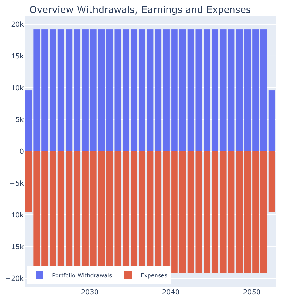
In the left overview, below the horizontal axis in red, the annual expenses appear, which result from our $1.600 per month. If desired, you can also switch off “Binning of earnings and expenses into years” and see directly the monthly values. Above the axis in blue the portfolio withdrawals necessary for the expenses appear. In our simple example, we have to cover all expenses by portfolio withdrawals, so the diagram looks rather boringly symmetrical, since the withdrawals then always correspond exactly to the expenses:
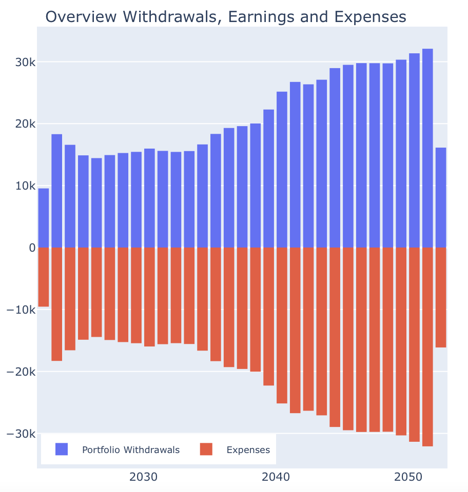
But why are expenses and withdrawals not constant over time but rather look like a crooked guitar? This is because we have set the switch “Expenses increase with Inflation” by default. I.e. we tell the simulator that our monthly expenses should increase with inflation and thus their real purchasing power should be preserved. Therefore, the nominal expenses are displayed, which grow with inflation. In particular we always use the historical inflation rates that exactly correspond to the return values used to calculate the portfolio development beside it. And usually the historic worst-case leading the minimal portfolio value at the end is shown. So to keep in mind: In the simulator, not only the historical returns but also always the corresponding historical inflation rates are considered in the calculation. This is not just an arbitrary design decision either. Returns and inflation rates are, of course, never independent of each other in economic terms either. Rather, central banks try to influence inflation with their interest rate decisions, and in doing so, they also accept effects on stock market returns. In the development phase of this tool, I also worked with constant inflation rates for the planning of expenses, especially in the beginning, because they are wonderful for running through different inflation scenarios. I presume that almost everyone who does their FIRE planning in Excel has a constant inflation parameter built in for their expenses. But when you start thinking about what inflation rate to consider for converting real to nominal returns for your stock portfolio, you run the risk of becoming inconsistent: If one takes the constant inflation rate, it usually no longer fits the economic situation of the respective real returns, if one takes the real historical inflation rate, it no longer fits the constant inflation in the spending plan. For me, therefore, I ultimately decided to completely dispense with constant inflation rates and always consistently use only the historical inflation rates. Therefore the graph looks like it is.
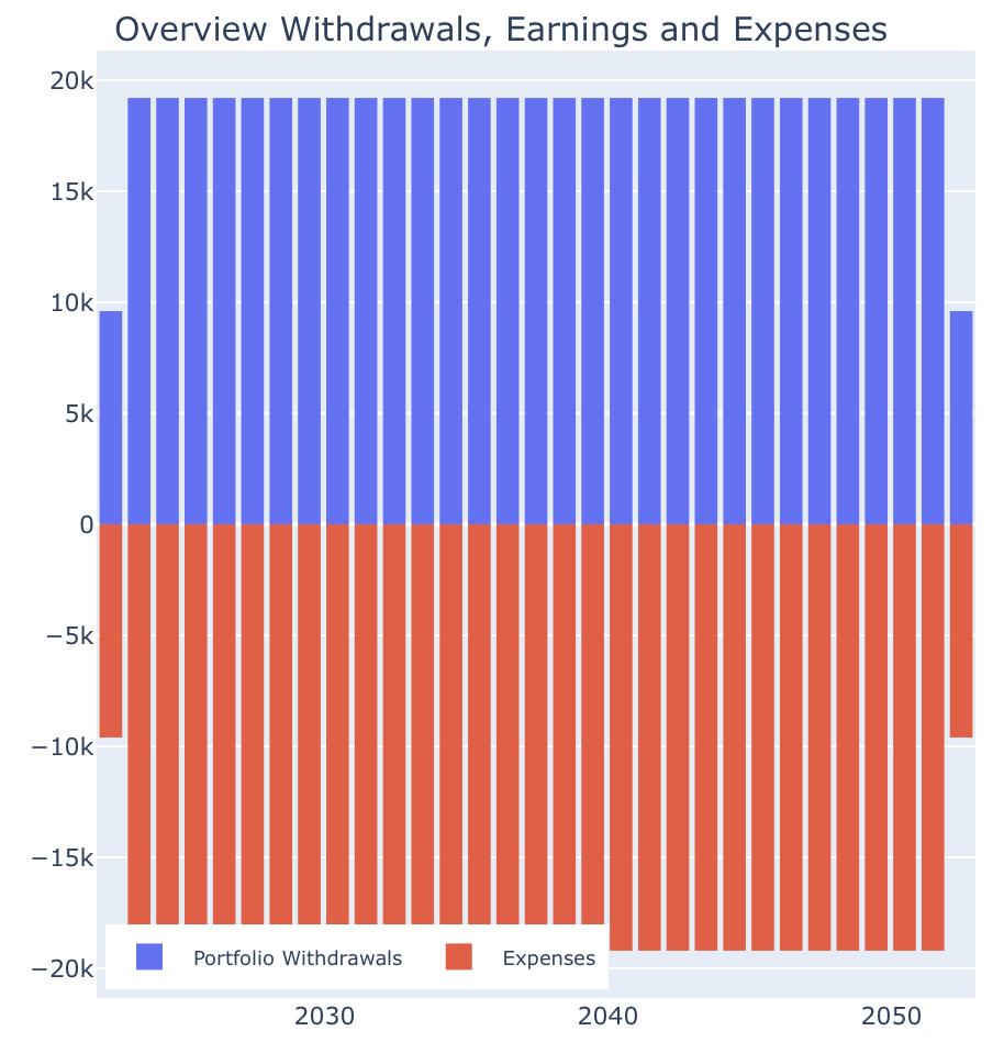
If you take out the switch “Expenses increase with Inflation”, the picture becomes even more boring: The expenses remain then also nominally constant and the necessary portfolio withdrawals likewise (However, one should not expect to be able to fill the car with gas using these $1,600€ in 2050, but I digress …):
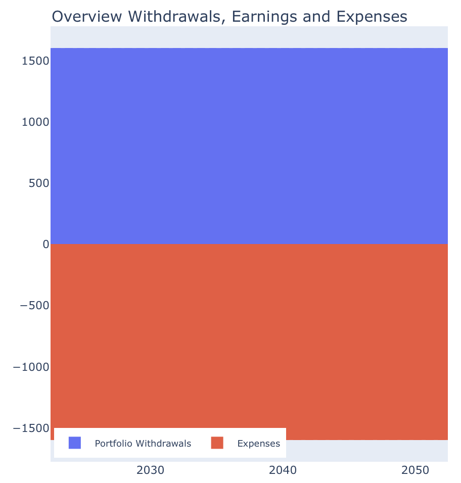
The deviating bars in the year view are simply due to the fact that the simulator always calculates from the current month of this year and thus the first and last calendar year of the simulation are not complete. In the monthly view, therefore, it looks quite trivial:
Nominal or real representation of the portfolio development over time
After explaining if, why and which inflation we take into account, we are now ready to press the next button. This one is labeled “Real Monetary Values w/o Inflation Effect” and hides the effects of inflation again in all charts on this tab. I.e. after setting this switch, everywhere instead of the nominal values the purchasing power adjusted real values are displayed and in the monthly view we now see the following picture:
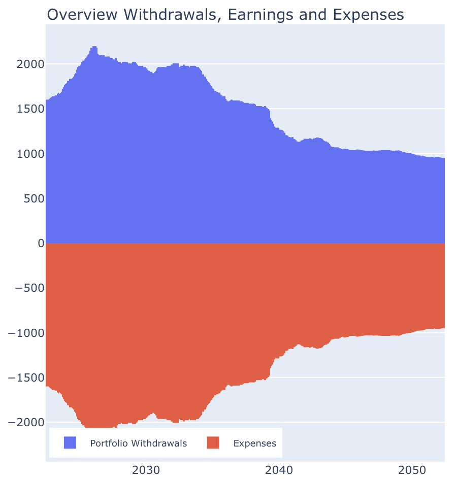
Oops, real expenses suddenly become smaller over time! We remember: Above, we have removed the switch “Expenses increase with Inflation” and thus accepted that the real purchasing power of our expenses decrease over time. This is exactly what is now visible in this illustration.
If we want to fill up our tank in 2050 in exactly the same way as we do today, then let’s now ruefully put the switch “Expenses increase with Inflation” back on and see the following picture in the annual view at the end of this exercise:
Although this overview looks exactly the same as the second chart above, its content must be interpreted completely differently:
- At the top, we have left expenses constant in nominal terms, i.e. we completely ignored inflation, and we have plotted the trend in nominal terms.
- In the last chart, we have let expenses grow with inflation, but we have hidden the effects of inflation and have plotted the real values. It is important to be aware of this difference. I would recommend running the simulator in the default setting (i.e. “Expenses increase with Inflation” is set and “Real Monetary Values w/o Inflation Effect” is not set) at the beginning until you get a good feel for these effects.
Best-case is not always best-case.
Interestingly, the presentation of results can also have smaller side effects. To see this, we go back to the basic settings desribed above and now press the “Best Case” button. We see again the nominal portfolio development starting from the historical scenario of June 1932 with a final result of 17.5 M$.
Now we switch back to the display of real monetary values. By default, the simulator always jumps to the worst case first, because that is naturally the case we are most interested in. So we have to press the button “Best Case” again. Now we see the maximum portfolio end value of 8.1 M$. Wait, I had written above in the 2nd paragraph something about real 7.9 M$ in the best case? What happened here? The best-case scenario now corresponds to a virtual start in March 2009. We see here the case where the nominal best-case is different from the real one. This virtual start in March 2009 would have resulted in real values in a better outcome than the virtual start in June 1932, although the latter would have performed nominally better. Nominally the portfolio in scenario no. 1658 would have ended up “only” at 7.1 M€ compared to the 17.5 M€ of scenario 737. At this point, however, two concluding remarks are worthwhile:
If you have read carefully, you might have asked yourself how can you calculate a 30 year portfolio development with a virtual start date in March 2009? Unfortunately, my crystal ball does not reach into the year 2039, which would be necessary to do this. Therefore, I help myself with a technical trick: After the last available monthly return from the Shiller data, I start again with the first monthly return in January 1871 in order to be able to calculate the 30 years completely. This cyclical approach of course leads to a historical break and may affect the results somewhat. EarlyRetirementNow.com does this a bit differently: He calculates from this point on with a constant average stock return. This approach also necessarily leads to a break, but to me this seems potentially even more radical than my approach. However, anyone who has a better idea for solving this fundamental problem is welcome to email me at info@predict-fi.com. I would be glad to hear about your ideas.
Second note on the topic: The best case is actually relatively uninteresting, we are primarily concerned with the calculation of safe withdrawal rates that also cover a worst case if possible. In particular, the exact calculation of the withdrawal rates in the 2nd tab of the simulator calculates them for zero as the portfolio end value. And this portfolio value is both nominally and really zero, i.e. the difference between the two representations disappears there, so that this calculation is actually not affected by this representation effect.